
Pivot table is a report providing information, that cannot be easily recognized in original data.
In this tutorial we will use following table, representing cars from fictional used car dealership.
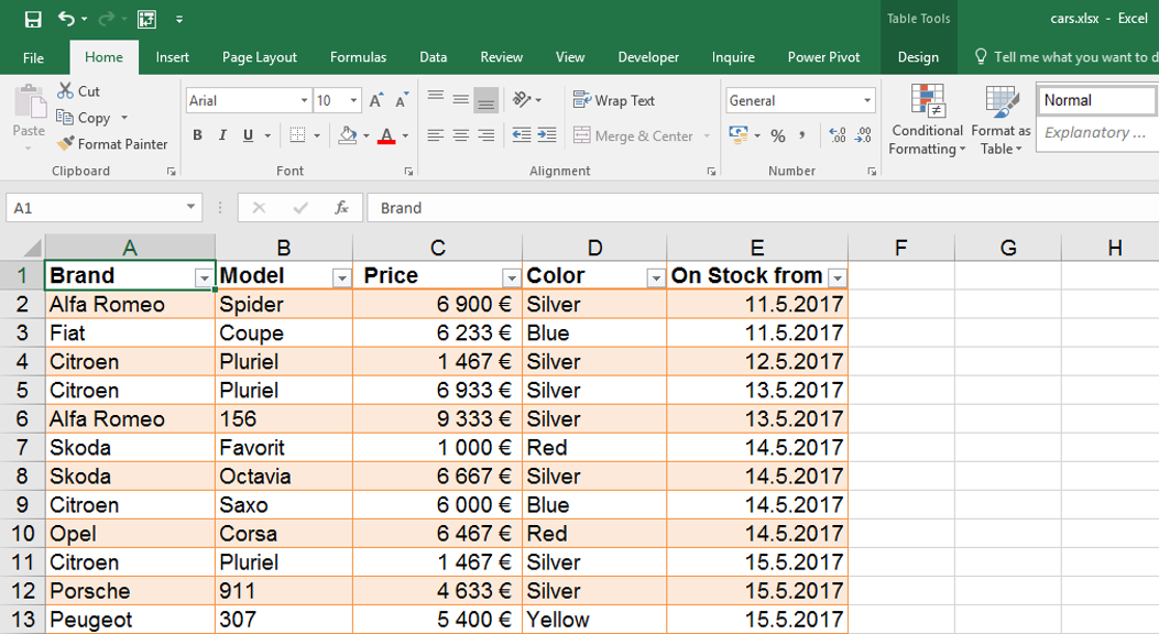
Thanks to the pivot table we can quickly respond questions like this:
- What are the total prices of various brands?
- How much cars were bought in which month?
- Are there any differences of average prices based on color?
- …
Now we will solve the first question – calculate the total prices of cars based on brands.
You can download the sample table here.
You can download the sample table here.
How to do it?
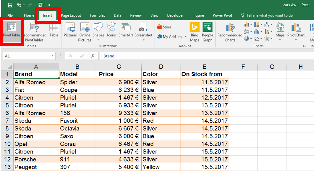
We will start by clicking anywhere into the table – there is no need to select anything more. Then we will click on Insert / Pivot table.
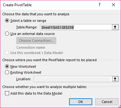
Following form can be left as it is and simply click “OK”.
Now new sheet with Pivot Table was created. There is no need to worry about the original data – the table with cars is still available on another sheet.
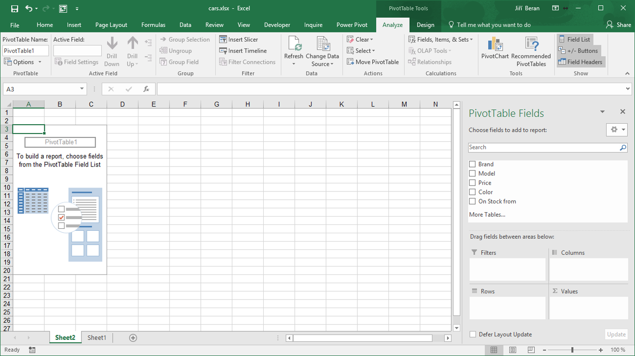
Let’s check the right pane with. There is a list of column headers from original data and four empty rectangles bellow them. The pivot table is created / modified by moving the headers bellow to one of these four places.
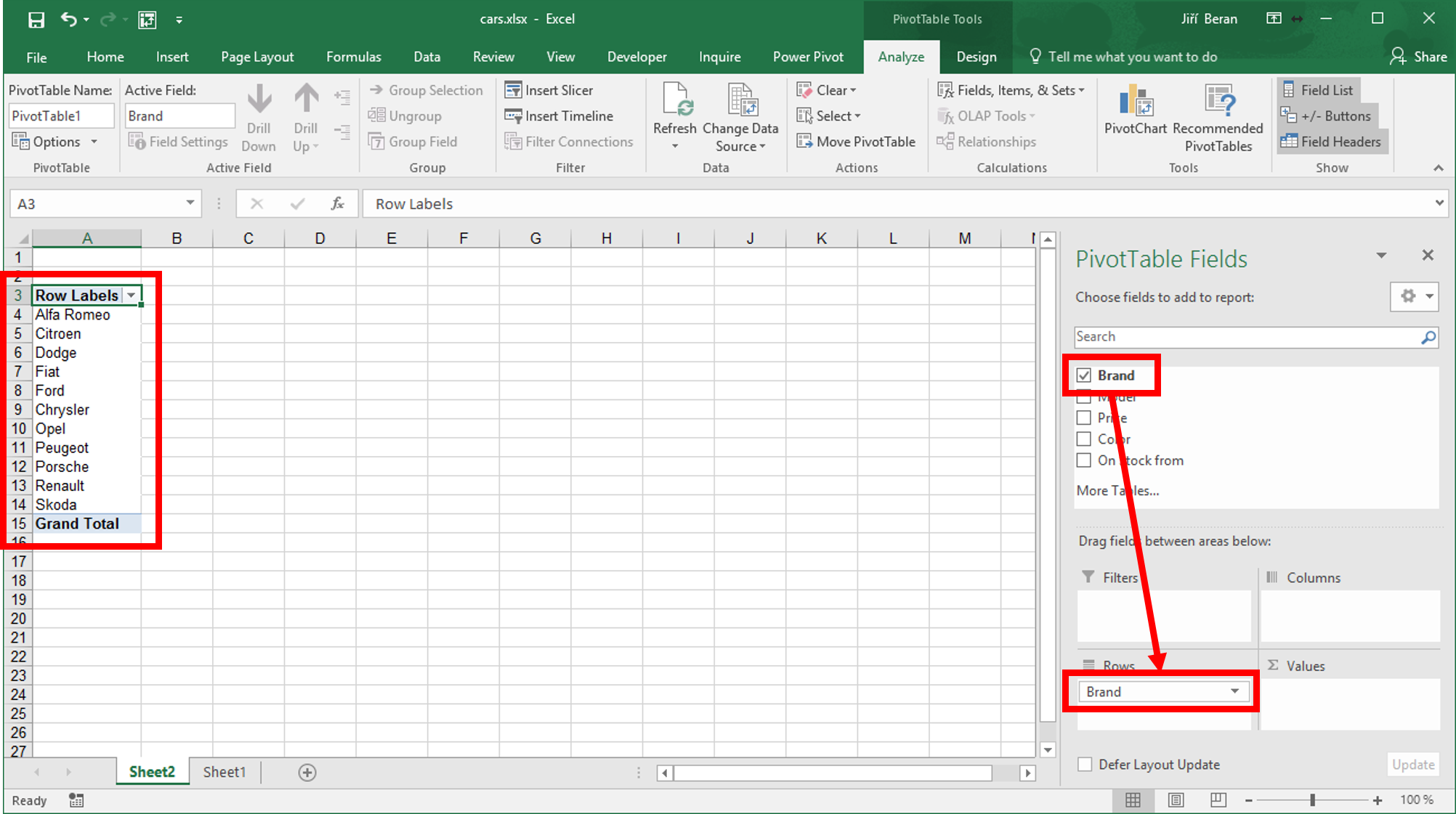
We wanted to see the total prices of cars, grouped by brands. So let’s move the “Brand” from upper list to the “Rows” rectangle. This creates the list of all cars on the left side of screen.
 Now we must find out the total prices. Lets move the “Price” to “Values”.
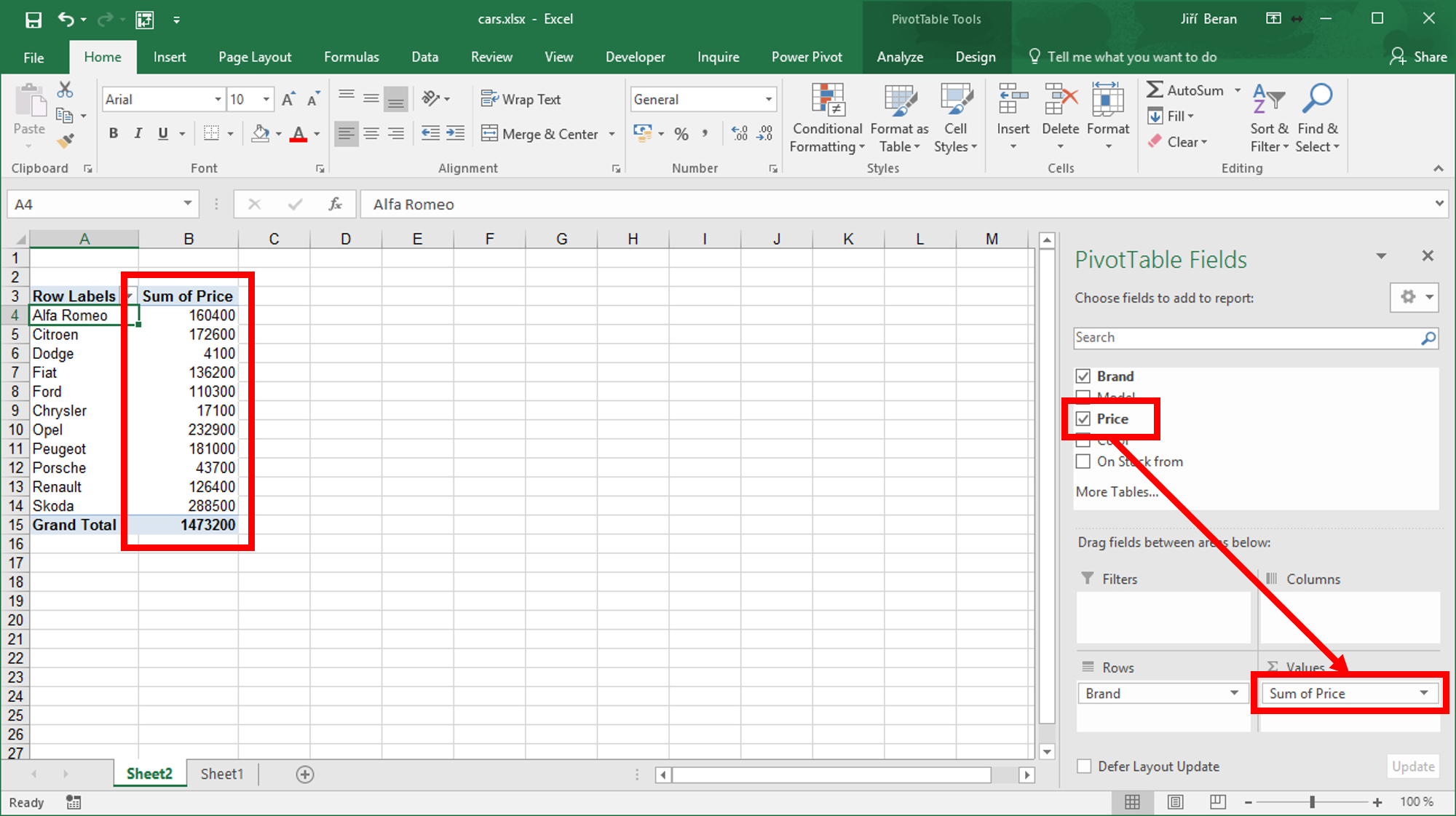 Now we can see the total prices for any brand present in original data and the original task is finished.
But what if we wanted to know how many pieces of which brand do we have? I mean not the total price, but the number of cars.
Let’s double-click on Sum of Price and in then select Count instead of Sum.

You can see this menu also when clicking Sum of Price / Value field setting in the right bottom corner of screen.
If you need both (sum and count), just drag the Price to Values two times – and one of them modify to Count.
Few tips:
- If the right pane disappears, just click to the report and the pane appears again.
- It is very easy to create a pivot chart from pivot table – just click on Chart icon and select the type of chart.
- More tutorials related to pivot tables