Comparison of two lists and finding differences

This article deals with a situation when you have to lists and need to find diferencies. In another words to find items, that are in one of the list and at the same time are not in another.

Example

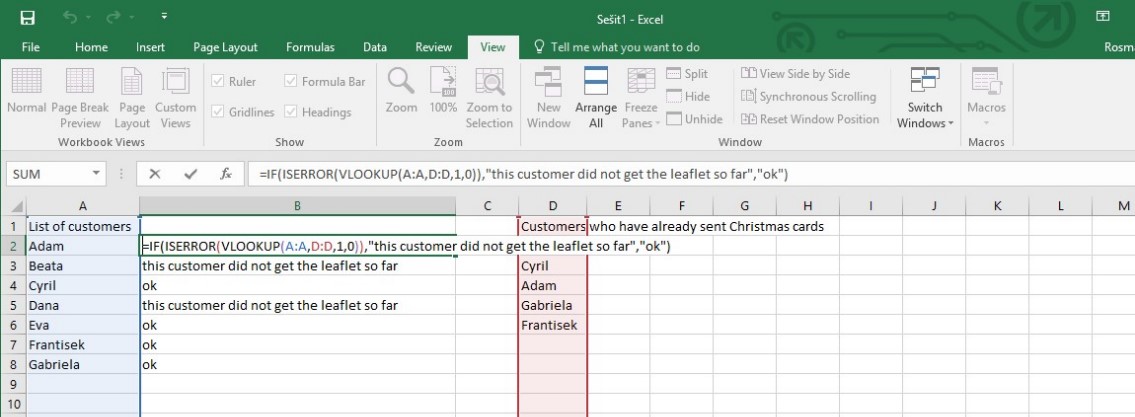
There are two columns with values (in two tables). I need to find the differences.

In the first column there are all customers. In the second column there are customers, that already got our new marketing leaflet.

Simply – in first column I need to highlight Beáta and Dana, because they aren´t in D column.

This searching can be done in more ways. In this article we will show tow of them – one using VLOOKUP function and other using COUNTIFS function.

VLOOKUP used for two lists comparison

We can go to B column and type this formula, trying to find values from A in D column.

=VLOOKUP(A:A;D:D;1;0)

We will use this formula for all column. In items from A, that are not available in D, the N/A appears. So these items are different in columns.

This solution is working, but definitely not nice. The result would be better, if we used this formula:

=IF(ISERROR(VLOOKUP(A:A;D:D;1,0));”this customer did not get the leaflet so far”;”ok”)

COUNTIFS used for two lists comparison

If you are not big fan of VLOOKUP, you can use COUNTIFS instead. COUNTIFS can calculate, how many times the value from A appears in D. 

The formula is quite short:

• =COUNTIFS(D:D;A:A)

or, with nicer result, like this (zeroes and ones are replaced by meaningful texts)

• =IF(COUNTIFS(D:D;A:A);”ok”;”this customer did not get the leaflet so far“)