Hypothesis testing

Author: Lenka Fiřtová

This article describes the principles of hypothesis testing. As an example, we will use “hypothesis testing for the mean”, but there are many different tests we can do. For example, the significance of correlation or the significance of regression parameters can be tested too.

One thing all hypothesis tests have in common is that we always have at our disposal a value calculated from a sample, and from this value we are trying to infer something about the general population.

For example, we might be interested in how many hours a day on average university students in our country sleep. The population is then all university students in the country. However, asking each of them how many hours they sleep is time consuming – there are thousands of students. Therefore, we usually proceed by asking a randomly selected sample, say a few dozen students, and then draw conclusions about the entire population from the sample data.

Example

A company has 100 employees. We think their average height is 175 cm. But is that true?

We don’t want to measure the height of all 100 employees. So let’s randomly pick 20 of them and measure only these 20. The results in cm are shown in the table below (for the sake of this example, the height of the remaining 80 employees is also written in the table in light grey – to represent the fact that we we don’t know these numbers, but these employees do exist).

It is easy to calculate that the average height of these 20 employees is only 173.75 cm, which is less than the 175 cm we had assumed. But is a difference of 1.25 cm large enough to say that our assumption of an average height of 175 cm is false? The hypothesis test will help us answer this question.

How to make a hypothesis

Let’s first clarify some terms. The population is all the employees of the company in question (100 people). The sample is 20 selected employees whose average height we know. A hypothesis is some assumption whose validity we are going to test. In our case, it is: the average height of the employees in the company is equal to 175 cm.

This statement is called the null hypothesis. The result of the test will be that we either reject it or we don’t reject it. The null hypothesis should be something like: ‘the variable in question is equal to a certain value’. It is usually denoted by H0.

We then formulate an alternative hypothesis to the null hypothesis. It is usually denoted by H1. Most often it is something like “the variable in question is not equal to a certain value”, but sometimes it is also “the variable in question is smaller than a certain value” or “the variable in question is greater than a certain value”. The first alternative hypothesis signifies that we are performing a two-sided test (we say that the variable in question can be either smaller or larger than our assumption), the other two alternative hypotheses signify that we are performing a one-sided test.

In our example, our null and alternative hypotheses are:

• H0: the average height of employees in the company is equal to 175 cm.
• H1: the average height of employees in the company is not equal to 175 cm.

So we are perfoming a two-sided test.

The point of a hypothesis test is to compare the so-called test statistic and the so-called critical value. The test statistic always follows a certain probability distribution – in this case, the Student’s distribution (which looks similar to the normal distribution).

We always perform the test on a certain significance level. The chosen significance level depends on how willing we are to accept the risk of an incorrect conclusion. Usually a significance level of 5% is used. At this significance level, there is a 5% chance that we will reject the null hypothesis even if it is true.

Test statistic

The test statistic is obtained by taking the calculated mean (173.75 cm) and change it in a way such that the result of the operation is a number from the desired statistical distribution – in our case, the Student’s distribution. This is because we can then compare this calculated number from the Student’s distribution with another number from the Student’s distribution – the critical value – and say whether or not our calculated number is “big enough”.

In our case, we calculate the test statistic by taking the difference between the measured value and the assumed value (173.75 – 175 = –1.25), dividing it by the sample standard deviation (using Excel or R, we find that it is 7.2) and multiplying all this by the square root of the number of values in the sample (20), i.e.: (–1.25 ∙ √20)/7.2 = –0.78. The test statistic is –0.78. For other hypothesis tests, the test statistic may be calculated in a different way, but the principle remains the same.

Critical value

The critical value is something like a threshold that determines if “the difference we have observed is big enough”. For example, if the average height of the 20 employees selected was only 160 cm, we would probably intuitively say that the difference from 175 cm is big. If it was 175.01 cm, we would probably intuitively say the difference is small. The critical value formalises this intuition into a clearly given number that is either exceeded or not exceeded. In our example, we will look for the critical value in the tables of Student’s distribution – see table below.

The Student’s distribution has one parameter: degrees of freedom. In our case, we will use a distribution with 20 – 1 = 19 degrees of freedom (always one less than our sample size). So we are looking for the row with the number 19.

What do the numbers inside the table mean? For example, the number at the top left, 1.376, which is at the intersection of row 1 and column 0.8, means that 80% of the values from the Student’s distribution with one degree of freedom are smaller than 1.376.

So what column is relevant for us? Let’s first take a look at what the Student’s distribution looks like. It is shown in the graph below. If we are using a 5% significance level, the critical value is the value from the Student distribution such that only 5% of the values lie further away from zero than that. When we do a two-tailed test, this means 2.5% of the values are greater than the critical value, and 2.5% of the values are smaller than minus the critical value. This is illustrated in the following figure: the red dot indicates the (as yet unknown) critical value.

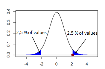
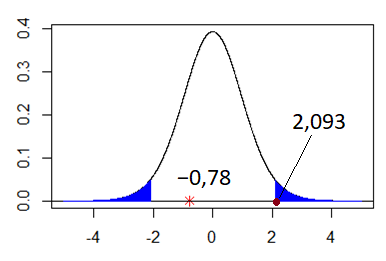
What number corresponds to this red dot? If 2.5% of the values are greater than the critical value, then 97.5% of the values are smaller than the critical value, so we are looking for the column with 0.975 in the heading. On the intersection of row 19 and column 0.975, we find the number 2.093. This is the critical value we are looking for. (We could also use the T.INV function in Excel: T.INV(0.975; 19) and not use the tables at all.)

Conclusion

All that remains now is to make a conclusion. The test statistic is –0.78. The critical value is 2.093. The absolute value of the test statistic is less than the critical value. In other words, the test statistic is not “far enough from zero”. Therefore, the difference between the calculated value from our sample (173.75 cm) and the assumed population value (175 cm) is not large enough (i.e. it is small enough to be attributed to chance).

Therefore, we do not reject the null hypothesis that the height of employees in the company is 175 cm.

Note that we can only reject or not reject the null hypothesis. We cannot confirm it!