Našimi kurzy prošlo více než 10 000+ účastníků
2 392 ověřených referencí účastníků našich kurzů. Přesvědčte se sami
This article deals with multiple way how to work with linear regression in Excel.
Linear regression is relation of two variables (=columns of data), when one depends on the second. This relation can be described by an equation y = a*x+b. In another words, when this relation is visualized in chart, it makes straight line. If you are interested in nonlinear regression, click here.
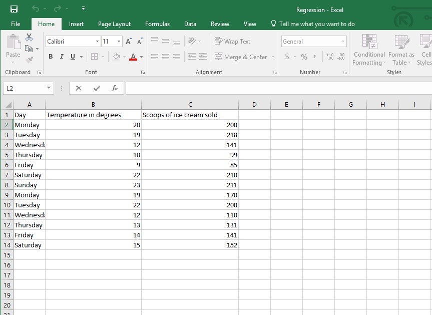
In this example we will deal with variables “number of ice cream portions sold in one day” (independent variable) and “average day temperature” (dependent variable). We will describe the equation of regression (find a, b parameters) and estimate, how many ice cream portions is going to be sold tomorrow, when the temperature will be 17°C.
For now we will not consider any factors except of ice cream portions and temperature.

The linear regression is described by equation y = a * x + b. In this case – number of ice creams sold = a * temperature + b.
X is an independent variable – which means variable, on which the second one is dependent. In my case the independent variable is a temperature – because the sales of ice cream depend on temperature. In another words the independent variable is on horizontal X axis.
Y is dependent variable – which means variable dependent on the other one. For now it is the ice cream sales, because it depends on temperature. In another words the dependent variable is on vertical axis Y axis.
There are multiple ways how to find “a” and “b”.
To be done.
LINEST works similarly to INTERCEPT and SLOPE, but it has to be used as a matrix formula. Which means select two cells, type =LINEST(C2:C14;B2:B14) and press Ctrl + Shift + Enter. The parameters a, b appear in the cells.
Possibly the most understandable way how to find parameters is their visualization. You can select all the table with headers and insert scatter plot. In a chart you can see the relation – if the points make some line.
Right click on some of the point and then “Add trendline”.
Select the proper trendline shape on the right pane and check Display Equation on Chart.
Now there is a line in chart, presenting the dependency.
There is also an equation I was looking for (if the Display Equation on Chart was checked). Now I know that a = 8,9707 and b = 14,166. This means if I take the temperature, multiply it by 8,98 add 14,17, I will have the estimated ice cream consumption.
Parameters a and b aren´t the only characteristics describing linear regression. If you need something more, you can use Analytical tools.
First of all we have to enable the analytical tools. Lets go to File / Options / Add-ins / Excel add-ins / Analytical tools.
Now we can see the Analytical tools in Data ribbon.
In Data / Analytical tools select Regression. In Y will be the values related to ice cream, in x will be the values related to temperature. The output contains many information, that can be difficult to interpret

Regardless which way was selected, the a and b characteristics will be the same. So if I knew that tomorrow should be 17°C, I can estimate the sale of 166,7 ice cream portions.
Download the data for practicing
2 392 ověřených referencí účastníků našich kurzů. Přesvědčte se sami
![]()
![]()
Pište kdykoliv. Odpovíme do 24h
© exceltown.com / 2006 - 2023 Vyrobilo studio bARTvisions s.r.o.