Use Power Query as a Pivot Table datasource

This article shows how to use Power Query to modify data for Pivot table or calculate values there.

Power Query enables us to change data (clean them, modify…) before Pivot table. In many situations it can replace (quite obsolete and limited) Calculated fields and Calculated Items.

It can be useful – since Power Query is a powerful tool.

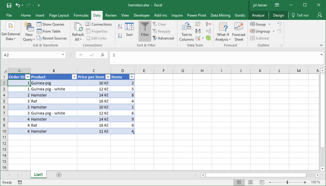
In this article we will use this source data:

to create this pivot table:

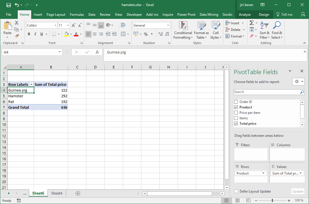
Notice, that the values in Pivot table are different from the source. There are two differences:

• Items “Guinea pig” and “Guinea pig – white” are merged to “Guinea pig”.
• In Pivot table there is total price – but there are numbers of pieces and price in the source.

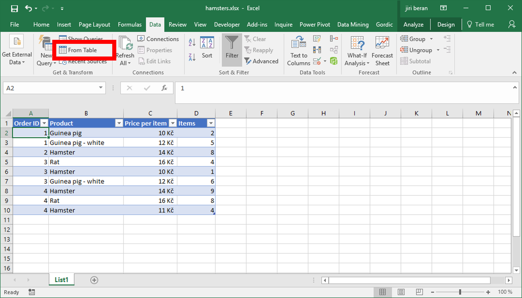
Let´s start. Click to the original table and then Data / From table.

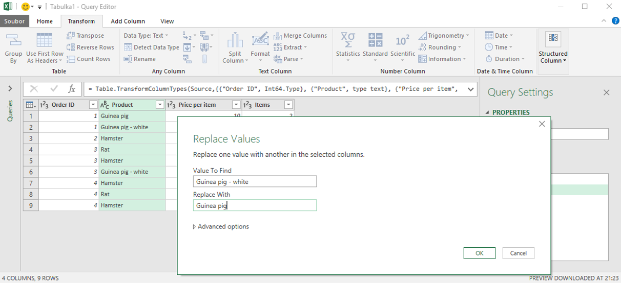
In Power Query editor make necessary modifications.

In Transform ribbon change the “Guinea pig – white” to “Guinea pig”.

Then select both number columns and click on Add Column / Standard / Multiply.

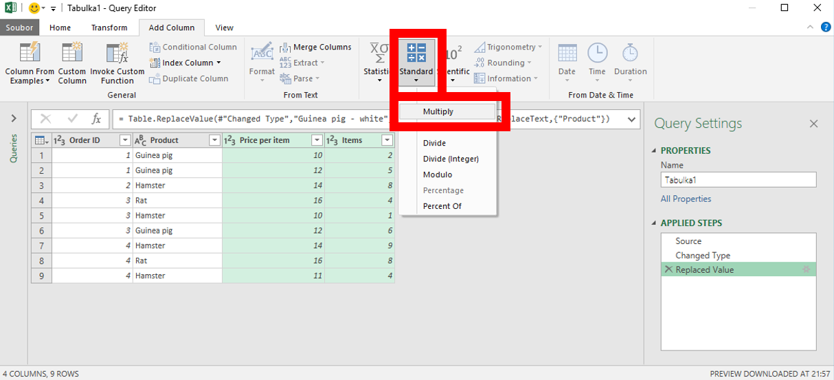
The new column can be renamed to Total price.

Confirm and go back to Excel (Home / Load and Close). 

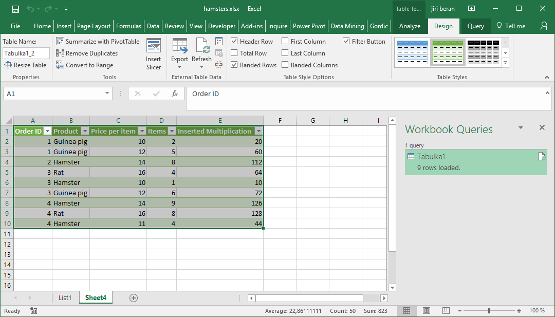
Now there is modified table, from which new Pivot table can be created.

Or, even better, new Pivot table can be created directly from query.

File can be downloaded from here