Pearson correlation coefficient in Power BI

In spite of there is no function like CORREL in DAX, the Pearson correlation coefficient can be calculated in two ways.

You can use the quick measure, or you can write your own calculation. In this tutorial there are both ways explained.

Pearson correlation coefficient in Quick Measures

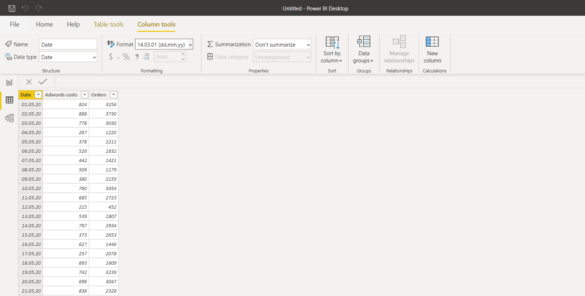
In this table, lets check the dependency of orders on Adwords costs.

Use the quick measure:

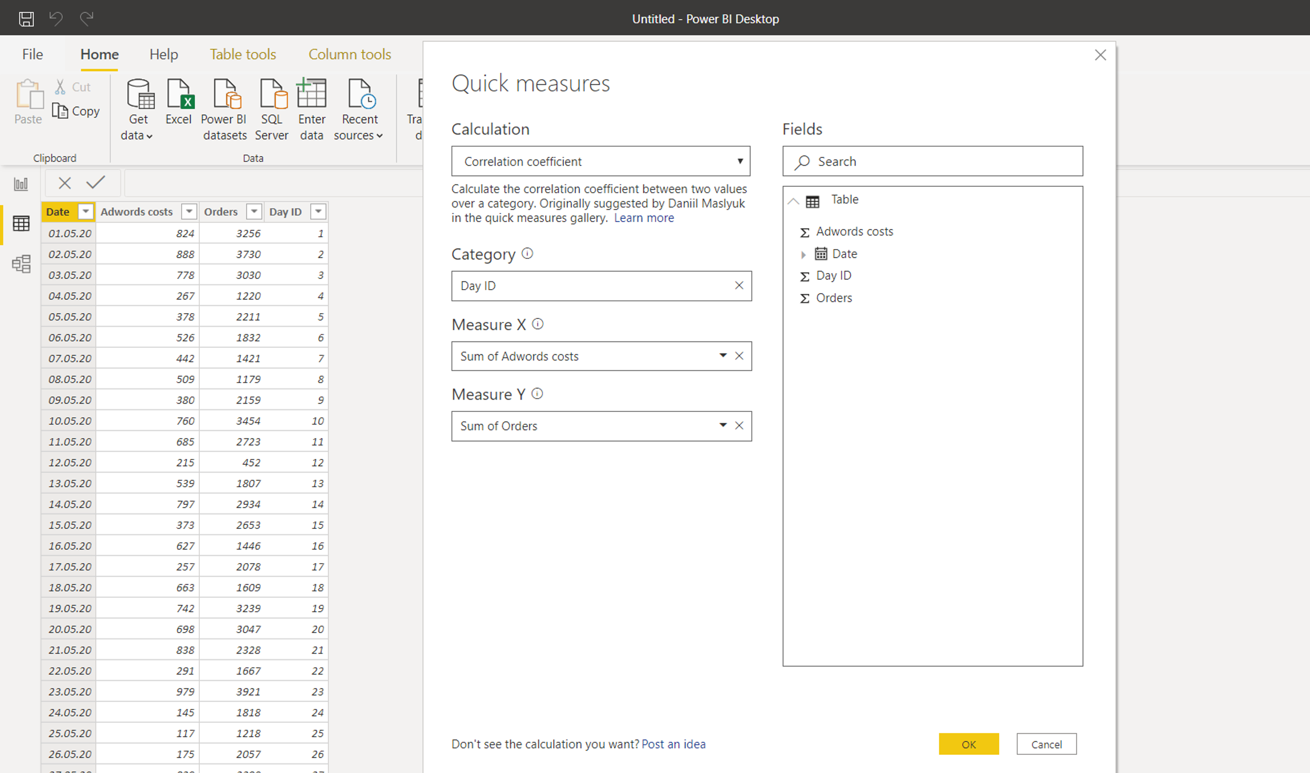
Quite complex DAX with variables appears:

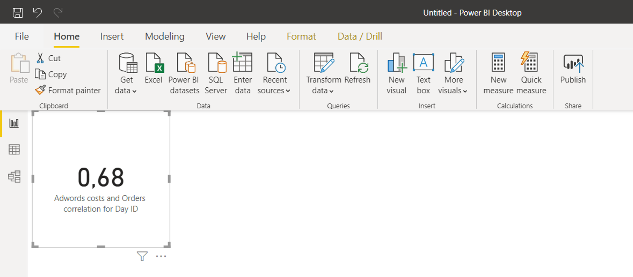
Then use it in some visualization:

Do it yourself (create your own formula and understand how it works)

The way described here is quite long and I´d really appreciate if you add something better to discussion.

I also have to remind that you can workaround this issue by publishing the data to Excel (and calculate it there very simply) or run R script on Power BI data, but both ways have some disadvantages.

So now we are going to work with this table containing two columns of data (spited into two groups A and B, that we can compare, but it is not necessary).

We will use this correlation coefficient formula:

I used three colors to highlight three parts of formula. They are going to be calculated separately in three columns, and then new measure will be calculated from them.

It sounds scary, but it won´t take more than few minutes.

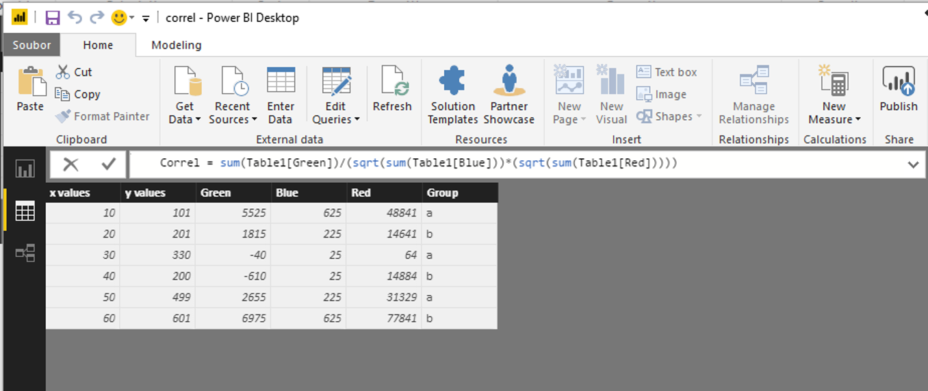
Here are the formulas for columns:

• Green = (Table1[x values]-average(Table1[x values]))*(Table1[y values]-average(Table1[y values]))
• Blue = (Table1[x values]-average(Table1[x values]))^2
• Red = (Table1[y values]-average(Table1[y values]))^2

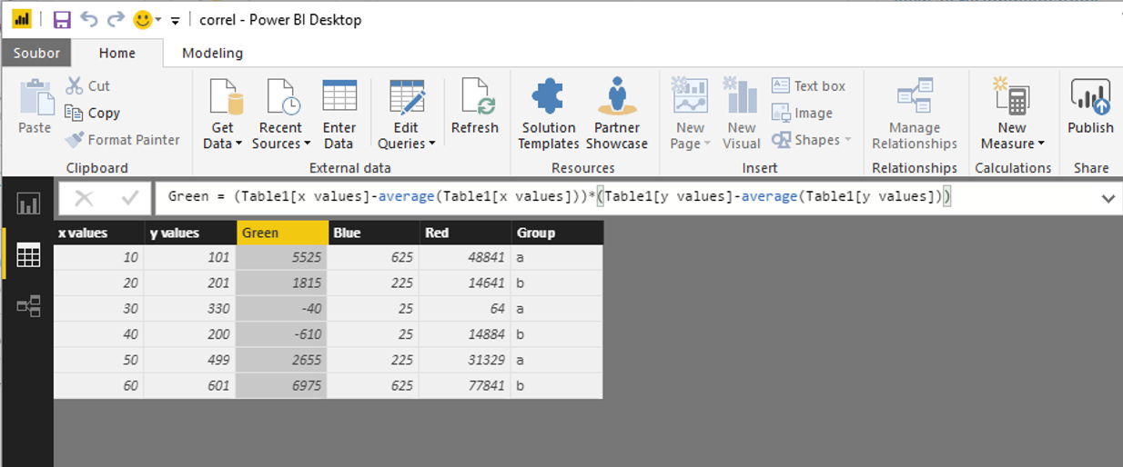
And this is the formula for correlation measure:

Correl = sum(Table1[Green])/(sqrt(sum(Table1[Blue]))*(sqrt(sum(Table1[Red]))))

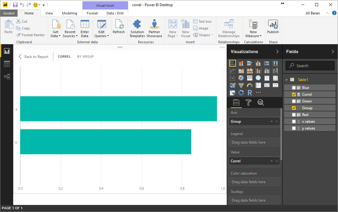
The values can be seen in visuals, where we can also compare both groups. Obviously, the A group is more correlated then B group.