Našimi kurzy prošlo více než 10 000+ účastníků
2 392 ověřených referencí účastníků našich kurzů. Přesvědčte se sami
Author: Lenka Fiřtová
This article explains the concept of correlation.
Correlation is a linear dependence between two variables (the word “linear” is important – variables can depend on each other in other than linear ways). The strength of the correlation is expressed by the so-called correlation coefficient, which takes values from –1 to 1.
It is important to point out that correlation is not the same as causality. If two variables are correlated, it does not necessarily mean that one influences the other. For example, it has been shown that the number of storks and the number of babies born in different European countries are correlated (correlation around 0.6). Does this mean that storks really deliver babies?
When we talk about correlation, we usually mean the so-called Pearson correlation coefficient. It is the covariance of the variables divided by the product of their standard deviations.
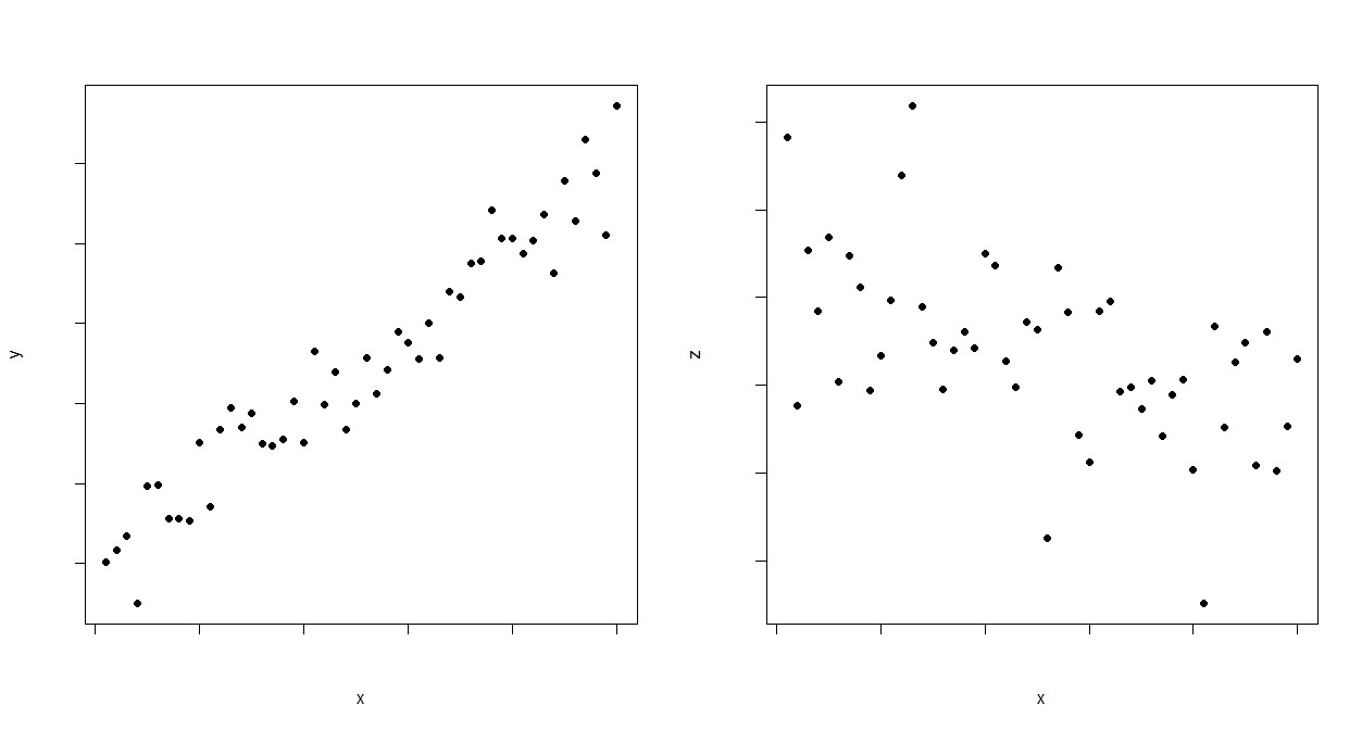
In the figure on the left we can see variables whose correlation coefficient is 0.96 (this is a strong positive correlation). In the figure on the right, we can see variables whose correlation coefficient is –0.54 (this is a moderately strong negative correlation; still, a trend of “the more – the less” is evident.
In a more complex statistical analysis, we can ask ourselves whether the correlation coefficient is large enough to conclude that there is indeed a relationship between the variables in question.
Consider an example: a retailer wants to know whether there is a relationship between the outside temperature and the amount of lemonade sold. For two weeks, he writes down what the average temperature was that day and how many litres of lemonade were sold.
He gets the following values:
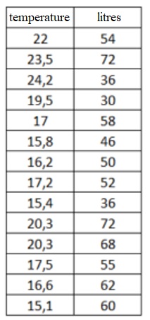
He calculates that the value of the correlation coefficient is 0.13 (here you can see how to calculate the correlation in R). And he asks himself: is there really a relationship between the temperature and the amount of lemonade sold, or did the correlation coefficient just happen to be like this during this particular period? In other words: is the value of the correlation coefficient really different from zero if we observe it over the long term?
If we were the retailer in question, how should we proceed? We should compare the so-called test statistic and the so-called critical value. The test statistic is a number that takes into account the calculated correlation coefficient and the amount of data we have available. The higher the calculated correlation and the more values we have available, the larger this number will be. The critical value is a threshold – a number from statistical tables that represents the minimum value that a test statistic must have so that we can say it is “large enough”.
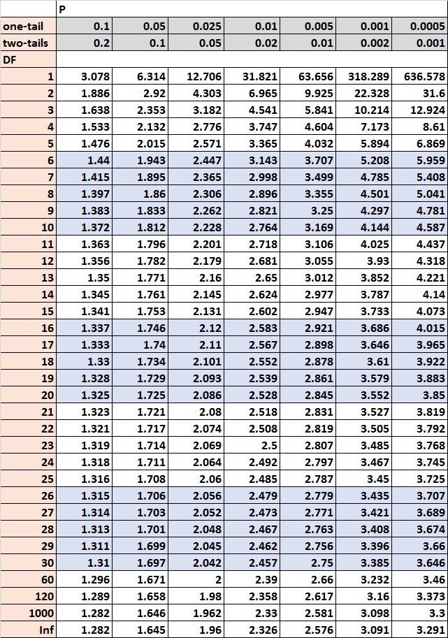
We need to determine the correct row and the correct column where to look for the critical value.
The row is based on the so-called degrees of freedom, which is the number of observations minus 2, in this case 14 – 2 = 12. The correct column is based on the so-called significance level. The significance level is up to us, most often we use a 5% significance level (the significance level reflects how confident we wish to be about the conclusion we draw: we look at the two-tails row). This leads us to a critical value of 2.179.
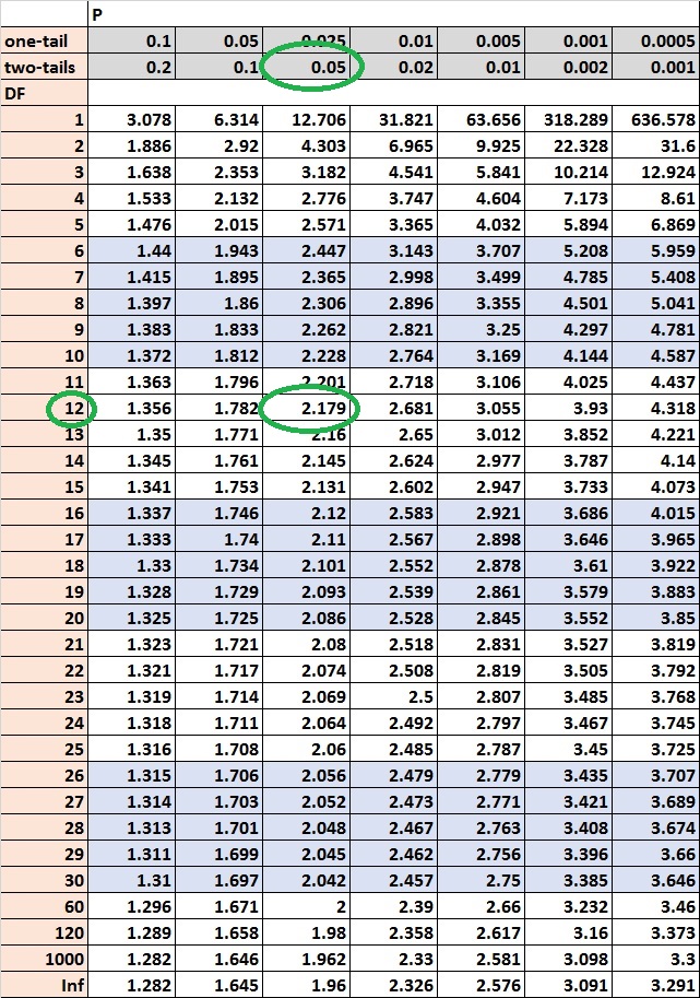
We compare the absolute value of the test statistic (absolute value because the test statistic can be negative) and the critical value. We can see that 0.45 is less than 2.179. Because the calculated test statistic is less than the critical value, the correlation is not significant. The test statistic is too close to zero to declare that there is a relationship between temperatures and the amount of lemonade sold. We would either have to observe a stronger correlation or try collecting more data (but even more data may not necessarily make the correlation significant).
On our website you can find articles on how to calculate the correlation coefficient in various programmes:
![]()
![]()
Pište kdykoliv. Odpovíme do 24h
![]()
© exceltown.com / 2006 - 2023 Vyrobilo studio bARTvisions s.r.o.